https://www.zcyphygeodesy.com/en/h-nd-139.html
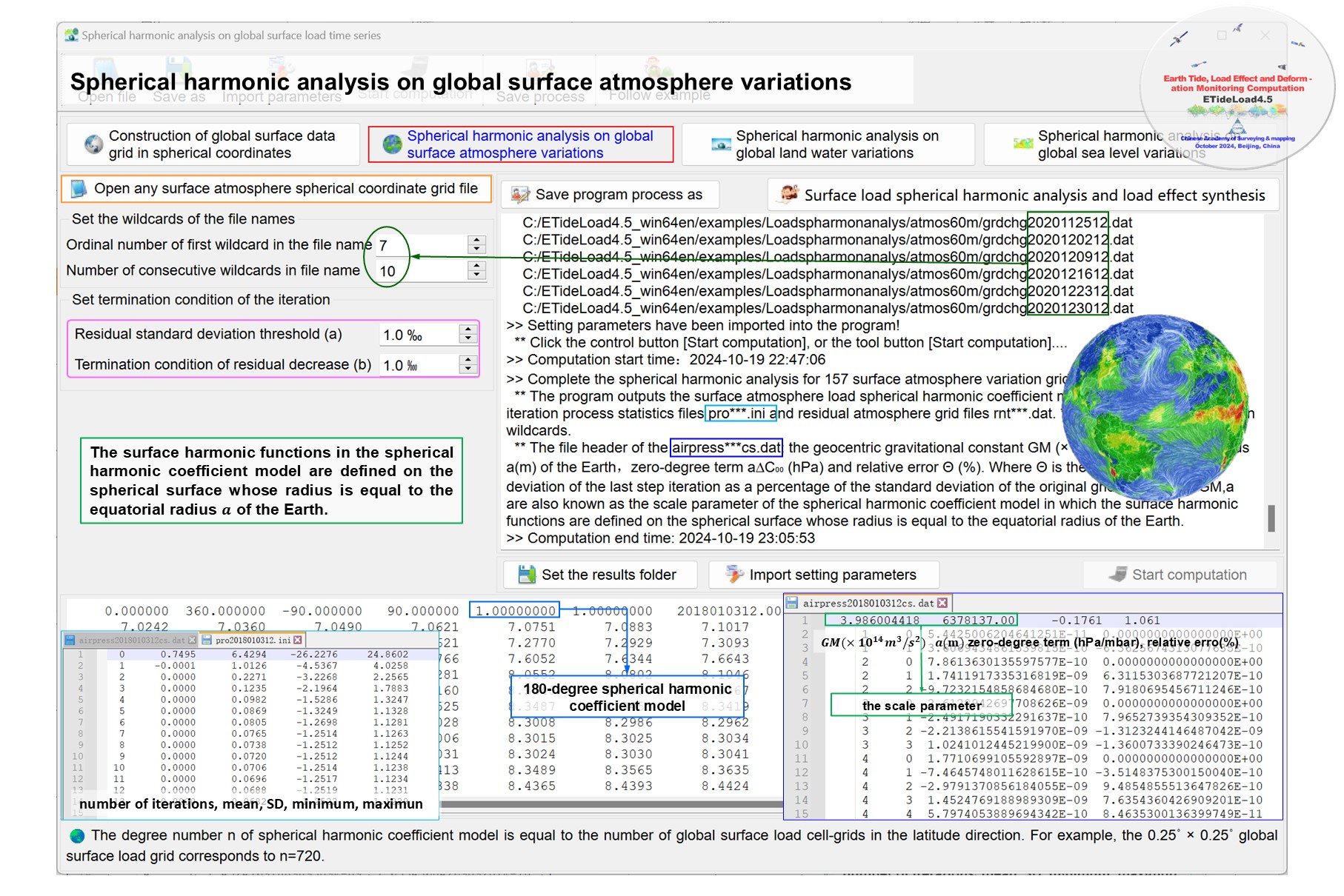
From the global load spherical coordinate grid model time series such as land/sea surface atmosphere, land water and sea level variation, construct the normalized surface load spherical harmonic coefficient (m) model time series by spherical harmonic analysis and calculate the load effect time series (Xcm, Ycm, Zcm, in unit of mm) on Earth's center of mass.
Using the model, the non-tidal load effects on various geodetic variations outside the solid Earth can be computed by the spherical harmonic synthesis.
The degree number maxn of spherical harmonic coefficient model is equal to the number of global surface load cell-grids in the latitude direction. For example, the 0.25˚ × 0.25˚ global surface load grid corresponds to maxn=720.
From the global surface load spherical coordinate grid model time series, construct the normalized surface load spherical harmonic coefficient (m) model time series by spherical harmonic analysis.

GobalharmonicanalysisLoad.f90
Input parameters: knd - =0 landwater EWH variation, =1 sea level variation =-1 surface atmosphere variation.
Input parameters: loadfl - = the data file name, in the file include all the load EWH spherical coordinate grid time series file names.
The seventh numerical value of load EWH grid file header is the long integer time agreed by ETideLoad.
Input parameters: dtmfl - = the land-sea terrain spherical coordinates grid file name. The land-sea terrain grid will be employed for land and sea separation, whose spatial resolution should not be lower than that of the surface load EWH grid.
Input parameters: kd, itd - iteration termination condition parameter. The standard deviation of the residual grid value is less than kd of the standard deviation of the original grid value, or the difference of the residual standard deviation of the previous step iteration relative to the current step iteration is less than itd of the standard deviation of the original grid values.
Loadharmanalysis(dtmfl,loadfl,knd,dk,itd)
Output time series files: the load spherical harmonic coefficient model time series files ***cs.dat, iteration process statistics time series files ***pro.ini and residual EWH grid files ***rnt.dat. Here, *** is the file name string of load EWH grid in loadfl with the last 4 characters removed.
The module outputs also the global load effect time series file geocenterairpr.txt on Earth's center of mass into the current directory. The record format: Epoch time (real years), Xcm (mm), Ycm (mm), Zcm (mm) and date (long integer agreed by ETideLoad).
SphHarmExpandFFT(ewh,hd,cilm,2,maxn,nlat,nlon,GRS)
Input parameters: ewh(nlat,nlon) - the load EWH variation grid (m).
Input parameters: hd(6) - grid specification parameters (minimum and maximum longitude, minimum and maximum geocentric latitude, longitude and geocentric latitude intervals of a cell grid, degree decimal).
Input parameters: GRS(6) - gm,ae,j2,omega,1/f, default value.
Return parameters: cilm(2,maxn+1,maxn+1) - 0~maxn degrees of load spherical harmonic coefficients.
SphHarmExpandFFT(ewh,hd,cilm,2,maxn,nlat,nlon,GRS)
Input parameters: cilm(2,maxn+1,maxn+1) - 0~maxn degrees of load spherical harmonic coefficients.
Return parameters: ewh(nlat,nlon) - the load EWH variation grid (m).
integralPnm.f90(legI,maxn,hd,lat)
Input parameters: lat - geocentric latitude (degree decimal).
Return parameters: legI(maxn+1,maxn+1) - the numerical integral of associative Legendre function.
BelPnmdt(pnm,maxn,t)
Improved Belikov recursion algorithm for pnm.
LegPn_dt2(pn,dp1,n,t) ! t=cos ψ
CAL2JD (IY0, IM0, ID0, DJM, J); JD2CAL(DJ1, DJ2, IY, IM, ID, FD, J)
PickRecord(str0, kln, rec, nn); tmcnt(tm, iyr, imo, idy, ihr, imn, sec)
mjdtotm(mjd0, ltm); tmtostr(tm, tmstr)
StatlsGrd(ewh,zero,nlat,nlon,pm,rst0);CGrdPntD2(lon,lat,dtm,nlat,nlon,hd)
Fortran90, 132 Columns fixed format. Fortran compiler. mkl_lapack95_ilp64.lib link library (include fftw3.f) required.
The rar compression package in the attachment includes the test project in visual studio 2017 - intel fortran integrated environment, DOS executable test file and all input and output data.


